

Calculated variables
Presentation of calculated variables
In the tab "Variable" one can identify easily the variables which one would like to receive in Insights. The variables (raw variables) that are received via a third system (hardware or other source) and the virtual variables (“calculated” variables) that are calculated via a combination a specific variable of the specific source with other data sources available in Insights. Please, make sure to read our "Best Practices" section before defining any calculated variable.
One can easily distinguish the raw variables from the virtual variables via a symbol indicated in the image here-under.
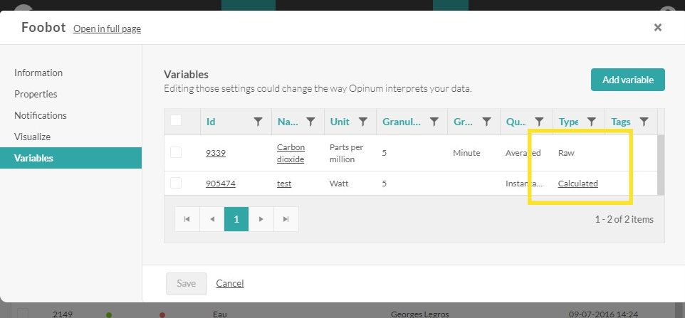
E.g. in this case the variable "Phase A consumption" is a variable indicating a consumption based on the raw variable received: "Phase A Index".
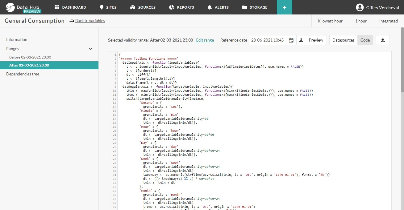
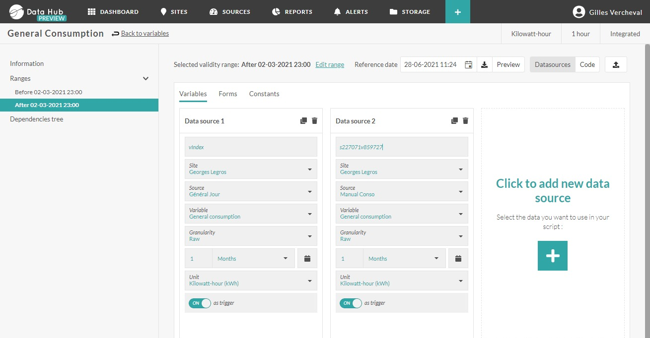
The interface for configuration is split in two parts:
At the left: one can see a configuration tool and select variables that will be combined via the calculation. In this case, one has indicated the sources which will be used to calculate a virtual variable. Apart from variables related to sources that are available in Verity, one can also define a constant value via the tab Forms.
At the right: the code permits to calculate the virtual variable based on the variables that are selected. In this case, the user uses a code in language R.
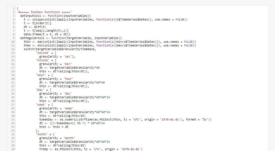
The code that is used by the client is a standard code in Verity. This code is a code to calculate the consumption based on index values.
The engine of the operation is stipulated in the section “Formula”:

We see that the result of the virtual variable will be calculated based on the successive difference of the index values.
The rest of the code is used for:
- Separate the different variables on an time axis (t$t), which will be used for the calculated variable (functions GetInputAxis, GetRegularAxis, SetDataOnCommonAxis)
- Filter the result of the calculated variables in order to ignore the points that are exactly the same as those that are already present in Verity (functions FilterNaOutput et FilterDuplicateOutput)
For more detailed explication on the functions and on the working method of the calculated variables, follow the link to the Webinar on the calculated variables:.
Here-under we provide some important notes in relation with the way to access the input variables.
If ‘x’ is the alias which is given to a input variable via the interface on the left:
- -inputVariables$x$TimeSeries$Dates permits to access the time axis from the input variable
- -inputVariables$x$TimeSeries$Values permits to access the values of the input variable
- -inputVariables$x$TimeSeries permits to access the table with two vectors referred to: at each time stamp, the value
The complete contract — every object the engine provides, and the exact structure it expects back — is detailed in Implement the calculation code.
In order to receive more insights on all the functionalities of the interface “Calculated variables”, image that we will calculate the consumption of a value starting from an index value:
Creation and use of calculated variables
Introduction
Imagine that we will calculate a virtual variable for consumption (which we call “Total consumption”) from an index value (which is called “Active energy” in this example. In order to start, one will click on "Add a new calculated variable" in the tab Config.
The following screen asks us to define a new calculated variable.
- Type of calculation: At this point, only language R is supported. The implementation of other languages is foreseen.
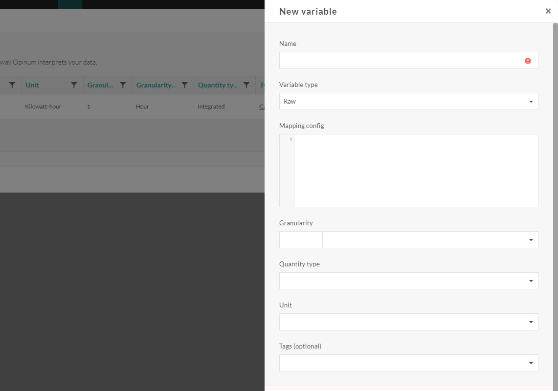
- Name: Name of the new calculated variable
- Unit: unit of the values of the calculated variables (when the calculation is performed). One should think about the grandeur of the results of the calculated variables so that the unit chosen is in line with the calculation.
- Granularity: the granularity of the variable indicates the time between each value of the calculated variable (e.g. hourly, daily).
- Quantity type:
- Instantaneous: characterizes an instantaneous variable which has a specific value at a moment in time (typical: stream, frequency, voltage, power, debit ...)
- Integrated: characterizes a variable from which the grandeur ensues from an integration (typical: energy consumption)
- Cumulative : characterizes a variable which will only accumulate (typical: a consumption index).
- Minimum: characterizes a variables from which the value will be the minimum value in a time interval (typical: minimum stream, minimum frequency, minimum voltage, minimum power, minimum debit, ...)
- Maximum: characterizes a variable from which the value will be the maximum value in a time interval (typical : maximum stream, maximum frequency, maximum voltage, maximum power, maximum debit, ... )
- Averaged: characterizes a variable from which the value will be the average value in a time interval (typical : average stream, average frequency, average voltage, average power, average debit, ... )
- When clicking on “Save”, the interface will switch immediately to the interface for the real configuration of the virtual variable:
Definition of the variables to include
A first step consists out of the definition to define the variables to include in the calculation.
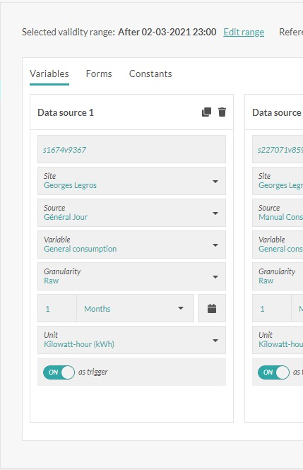
- Alias: name which will be given to the input variable in the calculation. This alias is used in the syntax: inputVariables$x$TimeSeries.
- Site: site to which the input variable is linked
- Source: source to which the input variable is linked
- Variable : input variable
- Granularity: by choosing "Raw", one chooses not to aggregate the values from the input variables. By choosing not for the option “Raw”, the input data will be aggregated based on your choice: minute, hour, day, week, month or year, before sending over the data to the calculation engine. ,
- Aggregation: if the granularity is not "Raw", one should choose the method of aggregation: sum, average, maximum, when appearing, variance or standard deviation.
- Period: the period permits to define the quantity of data input which will be send over to the calculation engine, at each new calculation. This period can be defined by using a relative manner (2 days before, the 10 latest measuring points,…) or by using a fixed manner by choosing dates via a calendar. How the period is positioned in time is described in How a calculation is triggered.
- Unit: the values of the input variable will be converted in the unit chosen, before sending the values to the calculation engine.
- As trigger: by activating these fields, one will assure that a new calculation will be performed each time new values of the chosen input variable are stored in Verity — one calculation per stored batch, see How a calculation is triggered. Verity recommends to always have this option activated for at least one variable, in order to ensure that the calculation engine is activated and the virtual variable will be calculated.
Following the same logic, one can use the forms or define a constant variable as input value. In order to do this, one has to define an alias and will select a from or define a value for the constant. The two icons permit to delete an input variable or to duplicate the values of the fields in another input variable.
How a calculation is triggered
A calculation is not run once per data point. It is run once per batch of data points stored on an input marked as trigger.
- When a set of points is stored in one go on a trigger input — for example a full day of quarter-hour readings — the engine runs one calculation for that batch, not one per point.
- Points of the same variable stored close together in time — within the ingestion time window, about one minute — are merged into a single batch, even when they come from separate deliveries. The batch then runs from the earliest to the latest of their timestamps, whatever the gap between them.
- Deliveries further apart in time trigger separate calculations.
- The code receives the whole window of each input in a single call, and every point it returns is written to the calculated variable.
Two dates position the window of every input:
| Date | Definition |
|---|---|
| Datapoint date | The timestamp of the earliest point of the batch that triggered the calculation, truncated to the minute. |
| Trigger date | The moment the calculation runs. When the datapoint date is later than that moment (a point dated in the future), the datapoint date is used instead. |
For a relative Period, the window of an input is then:
from = datapoint date − past Period
to   = trigger date + future Period
Without a future Period, the window ends at the trigger date itself.
A past window therefore does not stop at the received point: it always runs up to the moment of the calculation. All inputs are positioned on the same datapoint date, whichever input triggered the calculation.
Important
When old data is injected or corrected — a catch-up, a re-import, a late validation — the datapoint date lies far in the past, and every input is read from that date up to now. A calculation that reads a few points in normal operation can read months of data on a catch-up. The same applies when a single old point is stored within the same minute as recent data: the merged batch starts at the old point. Size the Periods, and plan re-imports, with this in mind.
The window is finally bounded by the validity dates of the formula and by the history and forecast limits of the account.
Future and Referenced Time Windows
In addition to the existing Period configuration, advanced time windows can be defined for input variables.
Future window configuration
When defining the Period, it is possible to specify a future-oriented window relative to the trigger date.
Supported options:
- Next X minutes
- Next X hours
- Next X days
- Next X weeks
- Next X months
- Next X years
Future windows can be combined with past windows.
Example — recent data
A point dated 17/09/2025 12:00 is processed at 17/09/2025 12:00: the datapoint date and the trigger date are the same.
- Past 7 days → 10/09/2025 12:00 → 17/09/2025 12:00
- Next 1 day → 17/09/2025 12:00 → 18/09/2025 12:00
- Past 7 days + Next 1 day → 10/09/2025 12:00 → 18/09/2025 12:00
Example — catch-up
A batch covering 01/09/2025 00:00 to 01/09/2025 23:45 is processed at 17/09/2025 12:00: the datapoint date is 01/09/2025 00:00, the trigger date is 17/09/2025 12:00.
- Past 7 days → 25/08/2025 00:00 → 17/09/2025 12:00
- Next 1 day → 01/09/2025 00:00 → 18/09/2025 12:00
- Past 7 days + Next 1 day → 25/08/2025 00:00 → 18/09/2025 12:00
Datapoint-based selections are not supported for future windows.
Input-referenced timeframe
Instead of defining its own period, an input variable can use the effective timeframe of another input variable.
In this case:
- The reference input defines the effective start and end timestamps.
- The dependent input retrieves data strictly within this same timeframe.
This configuration ensures precise alignment between inputs and avoids unnecessary data retrieval.
Time reference rules
The rules below use the dates defined in How a calculation is triggered.
- The past window starts from the datapoint date.
- The future window is counted from the trigger date:
- when the triggering point is dated before the moment of calculation (the usual case), the future window is counted from the moment of calculation;
- when the triggering point is dated after the moment of calculation (forecast data), the future window is counted from the datapoint date.
- "Future-dated" and "past-dated" refer to the point that triggers the calculation, never to the calculated variable itself.
Master / Slave behavior
When an input variable is configured to use another input as timeframe reference:
- If the master input uses a duration or absolute dates, the slave input uses the window computed for the master, after the formula and account limits have been applied.
- If the master input uses a number of previous points, the slave input is read between the first and the last point actually retrieved for the master. When the master returns no point, the slave falls back to the window computed for the master.
- A slave input can itself be marked as trigger. Its points then set the datapoint date, and the master's window is positioned from that date like any other input.
Example
A monthly coefficient (slave, trigger) references a quarter-hour consumption (master, last 10 points). A coefficient dated 01/09 and processed on 17/09 reads the 10 consumption points preceding 01/09 plus every consumption point from 01/09 to 17/09; the coefficient is then read over that same range.
Implement the calculation code
The second part consists out of the implementation of the code R which will feed the calculation engine.
Whatever the calculation does, it always sits inside the same contract: the engine hands your script a fixed set of objects, evaluates it, and reads one precise structure back. How you compute is entirely free; what comes in and what goes out is not.
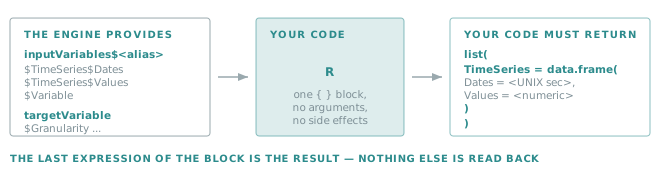
The script is a single R block, opened with { on the first line and closed with } on the last one. It takes
no argument and returns nothing explicitly: the value of the last expression of the block is the result, and
that value must be the list described in What your code must return.
What the engine passes to your code
Two objects are in scope, and they are the only data the engine hands over. Anything the calculation needs must therefore be declared as an input on the left panel first.
inputVariables — one entry per line declared in
Definition of the variables to include, addressed by its alias.
For an input aliased vIndex:
| Expression | Type | Content |
|---|---|---|
inputVariables$vIndex$TimeSeries |
data frame | The (timestamp, value) table for the whole retrieved period |
inputVariables$vIndex$TimeSeries$Dates |
integer vector | Timestamps, UNIX seconds, UTC |
inputVariables$vIndex$TimeSeries$Values |
numeric vector | Values, expressed in the unit chosen on the input |
inputVariables$vIndex$TimeSeries$Version |
character vector | Revision label, "" when none — see Versioning |
inputVariables$vIndex$TimeSeries$Tags |
character vector | JSON metadata, "" when none — see Tagging |
inputVariables$vIndex$Variable |
named list | Metadata of the input variable |
targetVariable — the definition of the calculated variable being produced. It is what allows the code to
build an output axis that matches the declared granularity, targetVariable$Granularity and
targetVariable$GranularityTimeBase being the two fields used for that.
Constants and forms declared on the same panel are addressed by their alias as well. They carry a single value rather than a time series.
Important
The data reaching your code is already transformed by the input configuration: aggregated to the chosen granularity, converted to the chosen unit, and restricted to the declared Period. Never re-implement any of those three in R — configure them on the input instead. The code sees the result, not the raw data.
Three properties of the incoming series are worth stating explicitly, because most defective calculations come from overlooking one of them:
- The series are not aligned. Two inputs have no reason to share the same timestamps, and neither has any reason to match the output granularity. Putting them on a common axis is a step of its own — see The anatomy of a formula.
- The series may contain gaps. A missing measurement is a missing row, not an empty one: two inputs covering the same period can have vectors of different lengths.
- Timestamps are UNIX seconds in UTC. Convert them explicitly with
as.POSIXct(t, origin = "1970-01-01", tz = "UTC")before any calendar reasoning — day boundaries, week numbers, daylight saving — and never assume the local time zone of the site.
Tip
Rather than guessing the exact shape of these objects, observe them. Click Download sample data, open the
data set in an R environment such as RStudio, and run str(inputVariables): you get the exact structure the
engine will pass, with the aggregation, Period and unit conversion already applied.
What your code must return
Golden rule
Whatever the calculation does, it returns one list, holding one data frame named TimeSeries, whose Dates and Values have the same length.
Nothing else is read back. A result that does not have this shape is not a partial result — it is a failed calculation, and no data point is stored.
The result is a list holding one data frame named TimeSeries:
list(
  TimeSeries = data.frame(
    Dates   = <integer vector, UNIX seconds, UTC>,   # required
    Values  = <numeric vector>,                      # required
    Version = <character vector>,                    # optional
    Tags    = <character vector of JSON strings>,    # optional
    stringsAsFactors = FALSE
  ),
  Errors = c()                                       # optional
)
| Column | Required | What is expected |
|---|---|---|
Dates |
Yes | The timestamp of each produced point, in UNIX seconds, UTC. |
Values |
Yes | One numeric value per timestamp, expressed in the unit declared on the calculated variable. |
Version |
No | One revision label per row. "" lets Insights apply its own default. |
Tags |
No | One JSON object per row, or "". Invalid JSON drops that row's tags only, without failing the calculation. |
Rules that matter:
DatesandValuesmust have the same length, and so mustVersionandTagswhen present. A mismatch fails the whole calculation.- The unit is not converted for you on the way out. The engine stores the numbers as they are, under the unit declared on the calculated variable at Introduction. Returning watt-hours into a variable declared in kilowatt-hours produces values a thousand times too large, and nothing will warn you.
- The granularity and the quantity type declared on the calculated variable describe what you return. If you return one point per hour, declare an hourly granularity; if the values are consumptions, declare the quantity type Integrated.
- Columns you do not need are simply omitted — do not return them empty.
data.frame()may turn text columns into factors. SetstringsAsFactors = FALSEand wrap text inas.character(...)wheneverVersionorTagsare involved.
Note
Returning an empty Dates / Values pair is valid: it means "this run produces nothing". This is the
normal outcome when the retrieved window does not contain enough data to compute a single point.
The simplest possible script
Not every calculation needs the full template. When there is a single input and the result keeps its timestamps
one-to-one, the whole script fits in a few lines. This one adds 10 to every value of an input aliased
vInput — copy it as it is and adapt the two marked lines:
{
  ts <- inputVariables$vInput$TimeSeries

  list(
    TimeSeries = data.frame(
      Dates  = ts$Dates,          # the timestamps of the input, kept unchanged
      Values = ts$Values + 10     # <- your calculation goes here
    )
  )
}
Replace vInput by your own alias, and + 10 by whatever the variable computes: * 1.05, / 1000,
pmax(ts$Values, 0), abs(ts$Values). Because Values is derived from ts$Values by an operation that
preserves the length, Dates and Values stay aligned by construction — the golden rule above is respected
without having to think about it.
Note
This script works because the result keeps the timestamps of the input. Declare the calculated variable with the same granularity as that input, otherwise the produced points will not land where Insights expects them.
Adding two inputs together is a different matter: two series have no reason to share the same timestamps, so the addition has to happen on a common axis. Start from the default code proposed by Insights — it already contains the toolbox, the axis block and the output filters — and replace the Formula line by:
result <- data.frame(
  Dates  = t$t,
  Values = regularVariables$vInput1 + regularVariables$vInput2
)
Both operands are then vectors of the same length, on the axis built just above.
The anatomy of a formula
The default code proposed by Insights is not one long calculation: it is four blocks that always play the same role. Recognising them is what makes an unfamiliar calculated variable readable, and what tells you where your own code belongs.
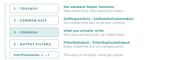
| Block | Functions | Role |
|---|---|---|
| Toolbox | GetInputAxis, GetRegularAxis, SetDataOnCommonAxis, FilterNaOutput, FilterDuplicateOutput |
The standard helpers, defined at the top of the script. Paste them once and leave them untouched. |
| Common axis | GetInputAxis(inputVariables), GetRegularAxis(targetVariable, inputVariables) |
Builds the time axis of the result — either the axis of the inputs themselves, or a regular axis derived from the granularity of the calculated variable. |
| Common axis | SetDataOnCommonAxis |
Projects every input onto that single axis, so the vectors become directly combinable. |
| Formula | yours | The one or two lines that actually compute the result, as a data.frame(Dates, Values). |
| Output filters | FilterNaOutput, FilterDuplicateOutput |
Removes the points that could not be computed, and those strictly identical to what is already stored. |
Once the inputs are on a common axis, they are available as plain vectors of equal length — this is the object
named regularVariables in the standard code, addressed by the same aliases:
t <- GetRegularAxis(targetVariable, inputVariables)   # t$t = the output timestamps
regularVariables <- SetDataOnCommonAxis(t, inputVariables)
regularVariables$vIndex                               # the input 'vIndex', on the output axis
Tip
The axis block becomes indispensable as soon as several inputs are combined, or as soon as the output granularity differs from that of the inputs: it is what guarantees that every vector has the same length and that the produced timestamps land on the declared granularity. Only a one-to-one transform on a single input can do without it — see The simplest possible script.
Worked example — a consumption from an index
The variable "Total consumption" is built from a single input aliased vIndex, which carries a cumulative
index. A consumption is the difference between two successive index readings, so the formula is one line:
Read from the inside out:
regularVariables$vIndexis the index, on the output axis.diff(..., 1)returns the successive differences — that is the consumption, but with one value less than the number of timestamps.append(..., NaN, after = 0)restores the missing length by puttingNaNfirst: the very first timestamp has no previous reading, so its consumption is undefined.data.frame(Dates = t$t, Values = ...)assembles the result on the axis built above.
That NaN is the point of the output filters: FilterNaOutput removes it, so the undefined first point is
never stored. The same reasoning applies to any calculation — produce a value for every timestamp of the axis,
mark as NaN the ones that cannot be computed, and let the filter drop them.
Writing the formula itself
The formula block is the only part that is genuinely yours. A few habits keep it correct:
- Think in vectors, not in loops.
a - b,diff(),cumsum(),pmin(),ifelse()all operate on the whole series at once. Aforloop over thousands of points is both slower and easier to get wrong on the boundaries. - Produce exactly one value per axis point. Any operation that changes the length —
diff(), filtering a condition,na.omit()— must be compensated so thatValuesstays aligned withDates. - Use
NaNfor "cannot be computed", not0. A zero is a measurement; aNaNis an absence, and it is removed before storage. Guard divisions accordingly:ifelse(d == 0, NaN, n / d). - Never widen the window from inside the code. If a calculation needs more history, extend the Period on the input — see The golden rule. The code cannot retrieve what was not delivered.
- Keep the code deterministic. The same inputs must always give the same result: a calculation is re-run
whenever a point is corrected, and a result that depends on
Sys.time()or on a random draw silently rewrites its own history. - Load only the packages you use. The list available on the Verity R server is given at the end of
this page, and every
library()call is executed at each calculation.
Common mistakes
Dates and Values of different sizes, usually after a diff() or a filter. The calculation fails as a whole.
The formula returns Wh into a variable declared in kWh. No error, just values a thousand times too large.
Two inputs combined index by index without going through the common axis. It works until one series has a gap.
Calendar reasoning applied to raw UNIX seconds. Daily totals end up shifted by the UTC offset.
Undefined points returned as 0. They are stored, and read downstream as real measurements.
Dropping FilterNaOutput / FilterDuplicateOutput stores undefined points and rewrites unchanged ones at every run.
Verification tool

The button "Check" permits to verify the syntax of your code in R.
The button “Visualize” permits to visualize the result via a graph showing the result of your code, based on the calculation.
If you observe a behavior which is not in line with your expectations, two possible intermediate solution can help to define the problem:
Once you defined all your input variables, you can click on "Download sample data" in order to download the data set you defined. This data set will be used in the R environment, as for example RStudio. This data set will be send to the calculation engine at each trigger (as defined). The aggregation parameters, the period and the conversion unit are already applicable on this particular data set.
You can as well make a direct export of you R code by clicking on “Add”. Your code will be directly be exploited in an R environment, like for example RStudio.
These two mechanisms permit to turn your calculation in an R environment with as goal, for example, to use a debug tool.
Best practices
This section explains how to reason about a calculated variable before configuring it, and how to keep that configuration efficient over time. The single most valuable habit is to size the Period of each input from the shape of the data rather than from the way it arrives.
The golden rule
Before opening the configuration screen, answer one question.
Golden rule
For one result point, at one given timestamp: which data do I need for that point to be sound?
Not "which data do I need in general", and not "what am I receiving". One point, one timestamp, and what is required around it. The answer is your Period.
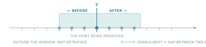
Insights runs one calculation per stored batch of points (see How a calculation is triggered). The Period you declare is the data made available before the earliest point of the batch — and, for a future window, after the moment of calculation. Sizing it on one output point guarantees that the first point of the batch has what it needs; the following points of the batch find theirs within the batch itself.
Tip
Write the answer down before configuring: "to produce the value at T, I need X before and Y after". A Period that cannot be justified in those terms is usually larger than necessary.
Size the Period on granularity
What matters is the granularity of the input — the gap between two consecutive data points — not the frequency at which files or messages are delivered. Consider an index metered every 15 minutes, delivered once a day:
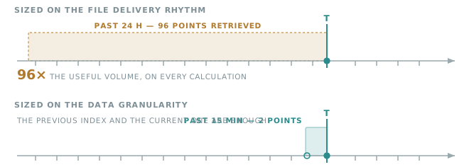
Both settings return a result. Only the second is sized on the data: computing a consumption from an index requires the previous point, so 15 minutes in the past is enough. The first retrieves a full extra day of history on every calculation, of which only the last point is used.
Granularity does come into play — but in second position, to turn a need into a duration:

Tip
An index metered every 15 minutes and delivered daily needs a Period of 15 minutes, not 24 hours. The delivery rhythm does not enter the sizing of the Period.
Choose the expression and the direction
Two decisions combine here, and each one has to be made explicitly:
- How the window is expressed: a relative duration, fixed calendar dates, or a number of previous points.
- In which direction it extends: towards the past, towards the future, or both.
In every diagram below, the vertical line is the timestamp being calculated and the shaded band is what gets retrieved. The diagrams show the steady state, where the received point is recent; on a catch-up, past windows extend up to the moment of calculation (see How a calculation is triggered).
The result depends on data on both sides — interpolation, centred averages, gap filling.
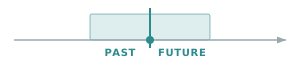
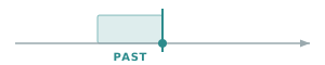
Nothing after the output timestamp is required. The most common case.
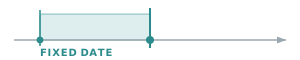
A fixed reference that never moves: a baseline year, a contractual starting point.
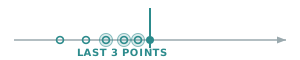
The need is expressed in points ("the last 3 readings") and the spacing may vary.
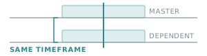
Several inputs must cover exactly the same range. See Future and Referenced Time Windows.
The wording of the business requirement usually settles the direction. "The last 24 hours" is a past window; "centred on the hour" needs past and future; "the reading before" is a single previous point.
Note
A window that extends into the future means the most recent results are computed from partial information, and will be refined as later data arrives. This is expected behaviour — make sure the users of the variable know it, so that a value changing after the fact is not read as an anomaly.
Share a timeframe between inputs
When several inputs must cover the same range, use the input-referenced timeframe rather than repeating the same Period on each one. One input acts as the master and defines the effective start and end timestamps; the dependent inputs retrieve data strictly within that same range.
Two benefits: less to fill in, and the ranges stay aligned when the master is later adjusted. Details and the master / slave rules are described in Future and Referenced Time Windows.
Triggering calculations
Calculations are triggered for every batch of data points stored on the source variables: one batch, one calculation, whatever the number of points it contains. For a calculation to run, the source variable must be marked as a trigger. Details in How a calculation is triggered.
Tip
Mark as "trigger" the inputs that carry the measurement the result depends on, and keep at least one so the engine is activated. Inputs holding slow-moving context data rarely need to be triggers.
Tip
An input whose values are regularly corrected or validated after the fact should be a trigger — that is what brings the corrections through into the result.
Historical and future data
When a calculation is triggered, each input is read from the datapoint date minus its past Period, up to the moment of calculation plus its future Period. Data stored after the received point is therefore always included up to now, whatever the Period.
Windows are also bounded by the data limits of the account: no further into the past than its history horizon, and no further into the future than its forecast horizon — 2 years unless configured otherwise.
Tip
Keep the data required by the calculation inside the forecast horizon.
Tip
Before re-injecting or correcting a long history on a trigger input, estimate what each calculation will read: on every input, from the oldest re-injected point up to today.
Note
Datapoint-based selections apply to past windows only; future windows are expressed as durations.
Cascading calculations
When a calculated variable is based on another calculated variable, a calculation is triggered every time a new batch of points is written by the source calculated variable.
Tip
Keep an eye on cascades: each level multiplies the number of calculations triggered by a single incoming batch. Review them whenever a new level is added.
Defining the calculation Period
The Period can be expressed in minutes, hours, days, weeks, months, years, or as a number of previous points.
Tip
Aim for the range the calculation actually consumes. A Period shorter than the need leaves out points that matter; a Period much longer than the need multiplies the volume retrieved on every calculation. The reasoning in The golden rule gives the right size directly.
Note
A Period expressed as N previous points retrieves the N points that precede the datapoint date plus every point between the datapoint date and the trigger date. N is capped at 1000. In normal operation this is close to N points; on a catch-up it can be far more.
Keeping the output consistent
The output granularity and unit deserve the same attention as the inputs.
- Keep the output granularity at least as wide as the inputs it is built from. A finer step adds intermediate points that carry no new measurement, and they will be read as measurements downstream.
- Check that the unit matches the quantity the calculation produces, and that the quantity type matches its nature. Changing the time step changes an energy (kWh); it does not change an average power (kW).
- Decide the timestamping convention explicitly. A consumption stamped at the end of its interval needs the previous point; stamped at the start, it needs the next one — the same requirement pointing in opposite directions.
Validating before going live
The verification tools described in Verification tool are the fastest way to confirm the reasoning above:
- Check validates the syntax of the code.
- Visualize shows the result of the calculation on a graph.
- Download sample data returns exactly the data set the inputs deliver to the engine, with the aggregation, Period and unit conversion already applied. This is the direct way to confirm that a Period retrieves what was intended.
Then review the boundaries, where behaviour differs from the steady state:
The first point has nothing before it. Observe what the calculation returns there.
With a future window, the latest points rest on partial information.
An input is missing over a period. Is the result absent, or produced anyway?
A day lasts 23 or 25 hours. Confirm each hour appears exactly once.
Change a value already processed and confirm the result is updated.
Compare against an invoice total, a manual reading, or an expected order of magnitude — chosen in advance.
Tip
Choose the reference to compare against before running the calculation. A reference picked in advance is what turns an impression into a validation.
Advanced configurations: date ranges and different calculations
Different date ranges can be defined for the same calculated variable, with a different calculation associated with each period or pivot date. This is the way to let a method evolve without recomputing history under the new logic: the earlier range keeps the rule that applied at the time.
Tip
Document each range and the reason it exists, so the configuration stays readable to whoever maintains it next.
Key takeaways
- One calculation runs per stored batch; its window starts from the earliest point of the batch and runs up to the moment of calculation.
- Size every Period from one output point, using the granularity of the input.
- The delivery frequency of the data does not enter the sizing.
- Decide the expression and the direction of each window explicitly.
- Share a timeframe between inputs with the input-referenced option rather than repeating it.
- Mark as triggers the inputs the result depends on, including those subject to later correction.
- Keep the future window within the forecast horizon of the account, and review cascades as they grow.
- Anticipate catch-ups: re-injected history is read up to today, on every input.
- Keep the output granularity, unit and quantity type consistent with what is produced.
- Validate with sample data and at the boundaries, against a reference chosen in advance.
Calculated Variable Engine Management
This section describes how to manage calculated variable engines in Insights Verity. Calculated variable engines are responsible for executing the calculations defined for calculated variables.
Manager
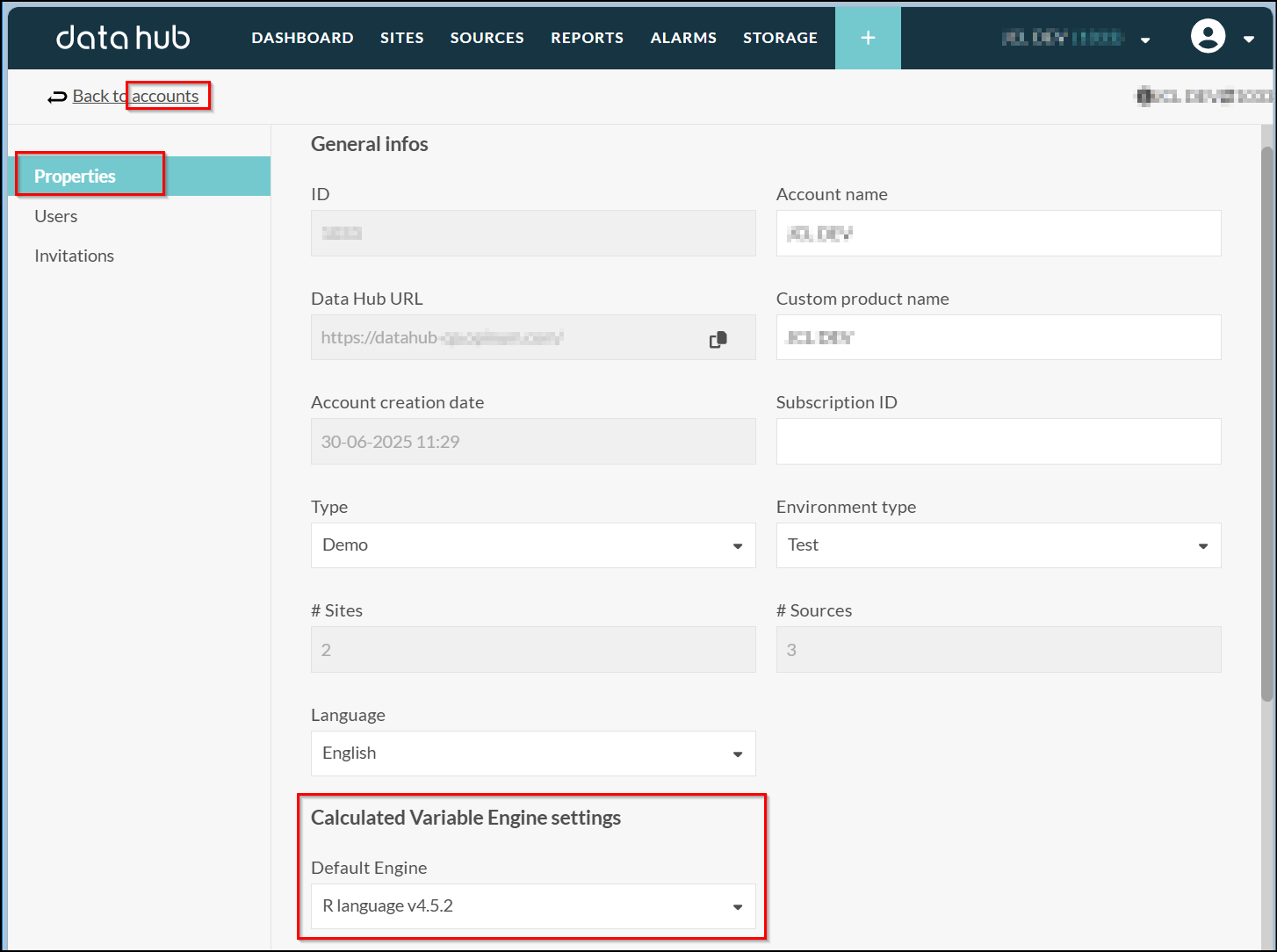
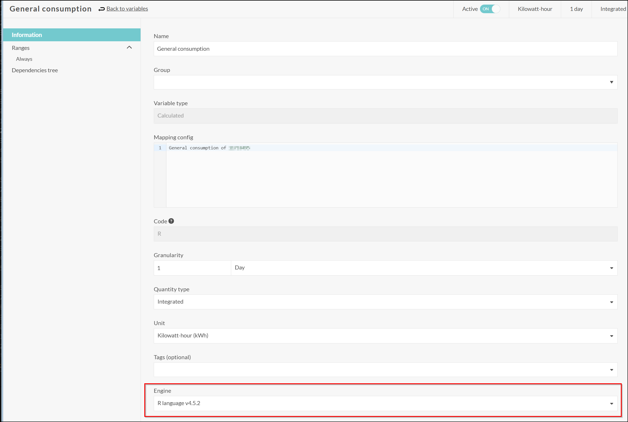
As manager, you have the ability to define default engines for new calculated variables or alter existing calculated variables to use a different engine :
Default engine: Go to properties of account and choose default engine for new calculated variables:
Specific: Go to information section of a calculated variable and choose engine for this variable:
Tip
Note: for more information about calculated variable engines hosted by Verity, please contact your Verity representative.
Administrator
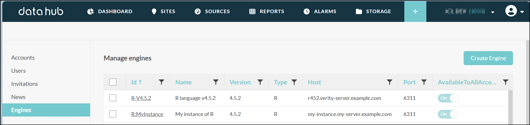
As administrator, you can configure new engines for calculated variables via the Admin interface.
Go to admin > engines to have a list of calculated variable engines. You can add a new engine by clicking on "Create engine" button.
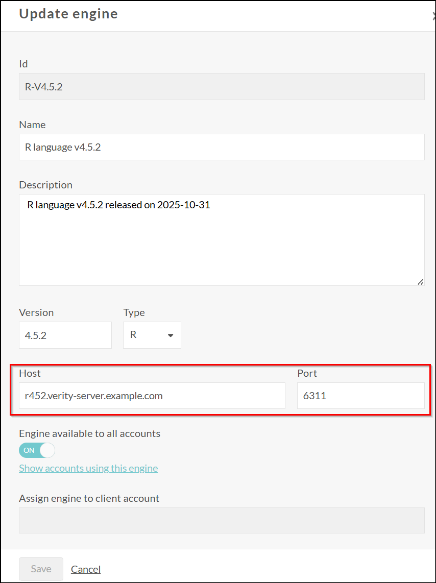
You can configure another R server on your infrastructure to be used as calculated variable engine by Insights Verity. So you can choose the best infrastructure for your needs.
Then fill in the form with the information of your R server:
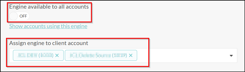
You can also configure the availability of the engine for specific accounts or for all accounts:
Tip
Note: at this time, only R engines are supported.
Installed packages on Verity R Server
For information, here is the list of the packages installed on the Verity R Server:
- RUN R -e "install.packages('Rserve', repos='http://cran.r-project.org')"
- RUN R -e "install.packages('ggplot2', repos='http://cran.r-project.org')"
- RUN R -e "install.packages('RJSONIO', repos='http://cran.r-project.org')"
- RUN R -e "install.packages('rjson', repos='http://cran.r-project.org')"
- RUN R -e "install.packages('Rmisc', repos='http://cran.r-project.org')"
- RUN R -e "install.packages('signal', repos='http://cran.r-project.org')"
- RUN R -e "install.packages('foreach', repos='http://cran.r-project.org')"
- RUN R -e "install.packages('doParallel', repos='http://cran.r-project.org')"
- RUN R -e "install.packages('jsonlite', repos='http://cran.r-project.org')"
- RUN R -e "install.packages('httr', repos='http://cran.r-project.org')"
- RUN R -e "install.packages('chron', repos='http://cran.r-project.org')"
- RUN R -e "install.packages('data.table', repos='http://cran.r-project.org')"
- RUN R -e "install.packages('quantmod', repos='http://cran.r-project.org')"
- RUN R -e "install.packages('oce', repos='http://cran.r-project.org')"
- RUN R -e "install.packages('RODBC', repos='http://cran.r-project.org')"
- RUN R -e "install.packages('base64enc', repos='http://cran.r-project.org')"
- RUN R -e "install.packages('lubridate', repos='http://cran.r-project.org')"
- RUN R -e "install.packages('dplyr', repos='http://cran.r-project.org')"
- RUN R -e "install.packages('forecast', repos='http://cran.r-project.org')"